It’s possible that you’ll need to excel find second largest value for various reasons. Today’s lesson will demonstrate how to use criteria to identify the second biggest value. Excel 2019 is what we are working with to run the meeting. You have the option of selecting the version that best suits you.
Before we go into the discussion, let’s take a moment to become familiar with the workbook for today, which will serve as the foundation for our examples.
We have a unique situation with Excel. Our employer continuously asked her to display the top three items, the bottom three nations, or we might need to find out who finished in second or third place in the competition. She would also ask her to present the top three competitors. She discovered that doing this task in Excel was rather difficult, so she was forced to manually sort the data, select the top three or bottom two items, and then copy and paste those numbers into the report.
In addition, this manual procedure needed to be carried out many times each week and each month. Therefore, this was a very inefficient use of time. In addition to that, she is not the only one… The majority of people who use Excel are unaware of the simple functionalities already built into the program and can do the task with only one click.
Therefore, she asked me whether there is a method to discover the second biggest value or the third largest value provided in a data set using Excel. She was specifically interested in finding the third largest value.
Using the Excel MAX function, you can quickly determine which data set has the ,greatest value and using the Excel MIN function; you can determine which data set contains the lowest value.
However, if you attempt to discover the second highest number or the third lowest value in Excel, you will find that the MAX and MIN functions cannot offer such a straightforward result. These formulas were formulated only supposed to be used for the greatest and lowest possible values. This is a really simple process. Simply utilize the method called Max(). if you want the least possible number, use the Min() function.
However, you cannot utilize Excel’s Min() or Max() functions to calculate the second biggest number when utilizing the same formula.
Excel Find Second Largest Value Using Large Function
It wasn’t until the late nineties that most people discovered a secret function in Microsoft Excel capable of doing the task correctly. It is referred to as LARGE.
For example, let’s imagine you have certain values in cells B2 through B6.
You might enter the following formula into Excel to get the number that is the Second Largest:
=LARGE (B2:B6, 2)
Without any further effort, this will provide you with the second-highest benefit.

The LARGE Function takes an array as its argument and returns the Kth greatest value contained inside the array. The syntax of the LARGE Function is =LARGE(array, k).
Therefore, you will need to add the following into the formula column of your Excel spreadsheet in order to identify the fifth greatest nation in terms of sales.
=LARGE (Data range, 5)
The LARGE function takes an array as its argument and returns the Kth greatest value contained inside the array. The syntax of the LARGE Function is =LARGE(array, k).
Therefore, what we can do is that will need to add the following to the formula column of your Excel spreadsheet to identify the fifth greatest nation in terms of sales.
=LARGE (Data range, 5)
Excel Find Second Largest Value Using Sumproduct
You may be already familiar with the LARGE function. This method returns the value in a list that is the nth biggest of those listed. We will need to utilize the LARGE function in conjunction with the SUMPRODUCT function to identify the first, second, third, fourth, and fifth largest numbers in a list depending on numerous criteria. Using these two functions together will allow us to do this. In various contexts, the SUMPRODUCT function is a great and really helpful tool to have available. It is often used to test several conditions simultaneously, such as in the example shown above.
The following formula illustrates how to determine the number the second greatest in a list where there are multiple amounts. The formula used will be “ =SUMPRODUCT(LARGE((B4:B9=G4)*(C4:E9),2))”
The sign for multiplication is used after each criterion, enclosed in parentheses, to guarantee that each criterion must be satisfied. For example, you might use the plus sign to apply OR logic between the checks in place of the minus sign.
It is of tremendous use to analyze data using formulae like this one. Before we introduced this, they reduced the amount of information in each area by utilizing three different PivotTables.
Step 1: Open an MS excel file and enter the data we are using for the Footballs Clubs and the cost of their Kit; from this data, we will be looking for the second-largest values from the list just by applying the formula and writing the name of the club in G3 Cell.
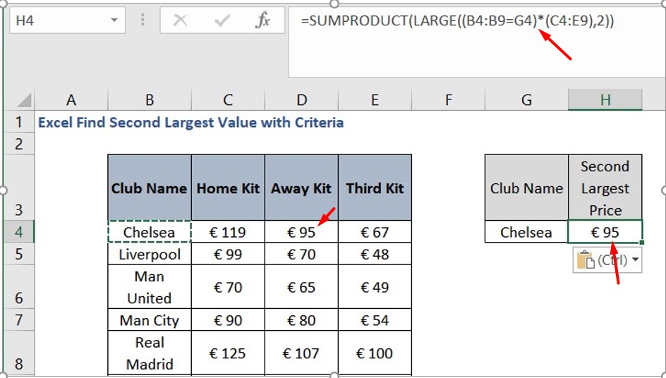
Step 2: Select the cell where you want the formula to show you the results and modify the formula according to your data set, and press enters to show you the results.
It is important to remember that the SUMPRODUCT function will be appropriate if you need to check numerous conditions.
Conclusion
You should now be able to discover excel to find second largest value. You can also determine the second greatest value inside a set of data that meets several different conditions. Using these functions, you will have no trouble determining which number in a list is the second biggest. Using these formulae, you may also search for the values that are the nth biggest; all you need to do is be aware of what could be altered. If you give these equations a little amount of practice, you’ll be an expert in no time at all.