Excel format cell based on Text is the most effective method for marking up individual results or marking results by trends. If you want to mark up individual results, utilizing excel’s format cell based on Text is useful.
However, creating the super reports requires more than simply saving the Text and the figures. There are many instances in which we are required to automate the report process to reduce the amount of labor required and increase the accuracy.
Excel gives us access to a wide variety of functions that, when applied to Text, provide helpful results and work. However, a few challenges remain, for which we will need to use certain strategies using the resources that we have accessible.
In the next sections, we will continue our education on conditional formatting by covering many more of its approaches. In Excel, TEXT refers to the collection of characters and string-like configurations of characters that transmit information about the various data and numbers. [ANSI] stipulates that each character has an associated code.
Text is made up of individual entity characters, which are the most basic unit discovered in Excel. This is the smallest piece that can be found.
We can carry out the operations on either the characters or the strings [Text].
Characters are not restricted to the letters A to Z or a to z, a large number of symbols are also present, as we will see in the next section of the article.
Excel’s TEXT data type is an inactive version of the number format. ANYTHING STORED AS TEXT [NUMBER OR DATE] WON’T RESPOND TO ANY STANDARD FORMULAS OR FUNCTIONS BUT SPECIALLY DESIGNED TEXT FUNCTIONS. [EXCEPTIONS DO OCCUR IN THE CASE OF NUMBERS]
If there is anything that has to be rendered inactive, such as the date being removed from the computation, we will put it in the form of a text. For the same reason, if we don’t want to do any computations for a number, we have to write it down as Text.
The practice of formatting in Excel based on the circumstances is called conditional formatting (CONDITIONAL FORMATTING). We can predefine several criteria inside the cell and then instruct Excel to format the data properly if one of those conditions is satisfied. The features of the Text, such as its font, size, and background color, are what makeup formatting. Formatting also includes the Text’s foreground and background colors.
Exact Function For Conditional Formatting
Let’s begin simply by first matching a text inside the data range and changing the format of that cell. Then, we will only need a bit of knowledge, and you will be able to do it in no time.
Step 1: Open Up a data sheet, enter the data, head over to Conditional Formatting In the Ribbon, and head over to the Equal To Function and Click. This will bring up a pop-up menu.

Step 2: Enter the Text you wish to highlight and choose the formatting from the drop-down menu, and you are set.
Using Custom Formula To Excel Format Cell Based On Text
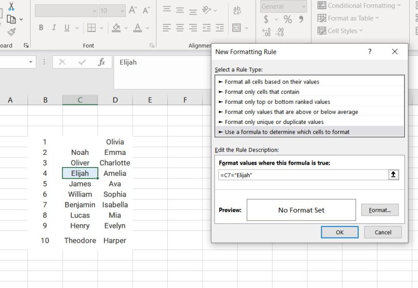
You can also employ a custom formula to use conditional formatting for cells. You will just have to add a new rule in conditional formatting and add in the formula you wish to match. We have used a relatively simple “=C7=Elijah” to change the formatting of that cell.
Step 1: Using the old data, select it, head over to conditional formatting, and select new rules. Next, select the Use A Formula To Select Which Cells to Format and enter the formula.
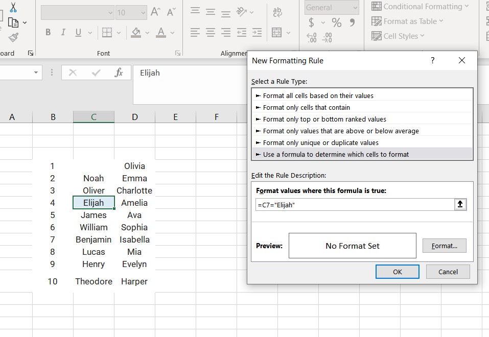
Step 2: Set the format options and press ok to see the results.
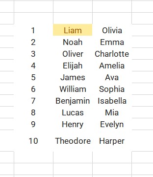
Using Exact Match To Excel Format Cell Based On Text
In this example, let’s figure out how to highlight the cells that contain the Text that is precisely the same as some other specified text, both in terms of the substance of the Text and the case in which it appears.
In this particular example, we will be using a data table to highlight the Text that fulfills the conditions that have been specified. We can also use the same approach to highlight the specific Text by applying conditional formatting on the provided List of the various data.
For example, we will choose the cell in which the name “Lucas” appears and highlight it. Keep up with the instructions.
Step 1: Choose all of the rows and columns, Go to the HOME TAB, then click Conditional Formatting, and then click New Rule. You may expect to see the following image when the dialog box opens.
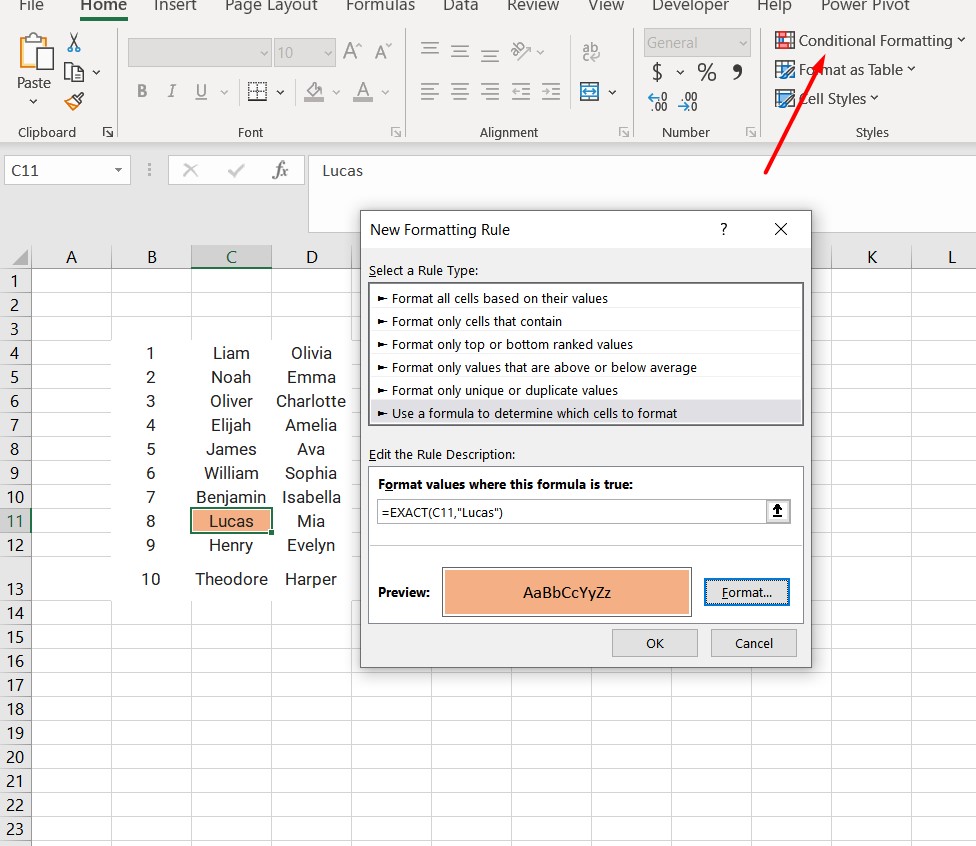
Step 2: To decide which cells should be formatted, choose the last option to utilize a formula. Input the formula =EXACT(C11, “Lucas”) into the appropriate field. Choose the format you want to use, and it will be used if at least one of the cells fulfills the criterion.
Conclusion
Now that you know the excel format cell based on Text, you can put this knowledge to good use in situations where you need to highlight certain names or where you want to highlight data that you need to evaluate. You can put this knowledge to good use in situations where you need to highlight certain names or where you want to highlight data that you need to evaluate. The strategies that we have shown to you are easy to understand and will greatly assist you. Because the formulas were established with novices in mind when they were being produced, they are not too difficult. However, you won’t be able to fully grasp these tasks unless you’ve put in the necessary amount of practice time beforehand.