This lesson walks you through a few different fast and simple techniques to cut gaps in Excel. Find out how to eliminate leading and trailing spaces and unnecessary spaces between words, as well as why the TRIM function in Excel is not functioning and how to repair it.
Are you comparing two columns to uncover duplicate entries that you are aware of, but your formulae are unable to locate even a single instance of this? Or, when you sum the numbers in the two columns, you keep receiving zeros when you check your total. And what in the name of all that is holy could be causing your accurate Vlookup formula to produce a plethora of N/A errors? These are just some of the many issues that you could be looking for solutions to. These problems are brought on by the presence of additional spaces before, after, or between the numeric and text values in your cells.
Microsoft Excel provides various options for removing whitespace and organizing your data in a more readable format. In this Excel lesson, we will examine the possibilities of the TRIM function, which is the quickest and simplest method to remove spaces from an Excel spreadsheet.
How To Trim In Excel From Left Using Trim
We can easily employ the trim function to clean out texts quite easily. The formula is quite easy “=TRIM(A1)” Use this “=TRIM(CLEAN(A1))” formula, for instance, to clear the contents of cell A1 of any extra spaces, line breaks, or other characters that aren’t wanted:
Step 1: Open up an excel sheet and enter the data where text is a cell in which you wish to get rid of the extra spaces there.

Step 2: Use the following formula, for instance, to get rid of the spaces in the cell A1:
Note that the TRIM function was developed specifically to eliminate the space character, which is represented by the number 32 in the 7-bit ASCII coding system. Please keep this in mind. If your data also includes line breaks and non-printing characters, you may erase the first 32 non-printing characters in the ASCII system by using the TRIM function and the CLEAN function. This will remove any unnecessary spaces that may be present in your data.
How To Excel Trim From Left For Whole Column
Imagine that you have a column of names and that, along with more than one space between each word, there is also some whitespace before and after the text. How exactly do you get rid of all of the leading, trailing, and unnecessary in-between spaces in all of the cells simultaneously? You may do this by duplicating an Excel TRIM formula along the column and then changing it with the appropriate numbers. The step-by-step instructions are provided below.
Step 1: Put the following formula into the uppermost cell, which is labeled A2 in our example:
=TRIM(A1)

Step 2: Put the cursor on the bottom right-hand corner of the cell with the formula (B1 in this example), and as soon as the cursor changes into the plus sign, double-click it. This will copy the formula down the column, up to the final cell that contains data. Consequently, you will end up with two columns: the original names, including spaces, and the trimmed names generated using a formula.
Step 3: Last but not least, the values in the first column should be replaced with the reduced data. But be cautious! It would be disastrous for your formulae to just paste the reduced column on top of the original column. To avoid this occurring, you should only copy values and not formulae while working with the data. How to do it:
- Select all of the cells that contain Trim formulas (B2:B8 in our example), then press the control key together with the letter C to copy the formulae.
- Select all of the cells that contain the initial data (A2:A8), then hit the Ctrl+Alt+V key combination, followed by the V key. The shortcut for Paste Values is what executes the Paste Special > Values command.
- Make sure you press the Enter key. Done!
How To Trim In Excel From Left From Numbers
You have just seen how the TRIM function in Excel successfully deleted all unnecessary spaces from a column containing text data without causing any problems. But what if the facts you have are numbers and not words? At first glance, it could seem as if the TRIM function has completed its task successfully. However, if you examine the trimmed values more closely, you will see that they do not act in a manner consistent with numbers. The following is a shortlist of abnormalities that may be present: Even after applying the Number format to the cells, the original column with leading spaces and the trimmed numbers remains left-aligned. This contrasts the standard alignment of numbers, which is right-aligned by default. Excel’s status bar shows just the word COUNT if two or more cells containing trimmed numbers are selected simultaneously. In addition, the SUM and AVERAGE should be shown for the numbers. When applied to the reduced cells, the SUM formula gives a result of zero.
To all appearances, the values that have been reduced are text strings when what we want are integers. You may correct this by multiplying each of the trimmed numbers by 1. (If you want to multiply all of the values at once, you can use the Paste Special > Multiply option.)
Therefore, the formula that we will employ is “=VALUE(TRIM(A2))”.
The above formula gets rid of any leading or following spaces, if there are any, and then converts the value that it produces into a number, as seen in the screenshot that follows:
Step 1: Open an excel file, enter the data, apply the formula, and press enter.

Step 2: Drag the autofill handle to apply the formula to the rest of the range. Check by doing the sum of numbers if the method works.
Trimming Leading Spaces For how to trim in excel from left
In some circumstances, you may need to enter repeated or even triplicated spaces between the words in your data to make it more readable.
Because you are well aware, the TRIM function removes any excess spaces that could be present in the center of text strings. However, this is not what we want to happen. We’ll be using a formula that’s a little bit more complicated so that all of the gaps in between are preserved:
=MID(A1,FIND(MID(TRIM(A1),1,1),A1),LEN(A1))
The location of the first text character in a string may be calculated with the help of the combination of the functions FIND, MID, and TRIM shown above. After then, you must provide that number to yet another MID function for it to return the complete text string beginning at the location of the first text character (the length of the string is determined by the LEN function).
Step 1: Open a data sheet, enter the new data, and apply the formula. Be sure to enter the ranges properly, and your data will be trimmed easily.
 easily.
Note: The Trim Spaces tool is what you should use if you want to get rid of the spaces at the end of the cells. There is no evident formula available in Excel to eliminate leading and trailing spaces while maintaining numerous spaces between words. Before you go in and remove spaces from your Excel sheet, it’s a good idea to check and see how many extra spaces are currently present in the file.
Find the overall length of the text contained in a cell by using the LEN function, then calculate the length of the string excluding the additional spaces, and finally, subtract the result of the latter calculation from the result of the first calculation: “=LEN(A1)-LEN(TRIM(A1))”
High Light Extra Spaces With the help of Conditional Formatting.
If you are dealing with sensitive or significant information, you may be reluctant to delete anything without first verifying what it is that you are getting rid of. In this scenario, you may begin by highlighting the cells that include unnecessary spaces, and after that, you can remove those gaps without risk. To do this, a conditional formatting rule should be built using the following formula:
=LEN($A1)>LEN(TRIM($A1))
Where A1 is the highest-level cell containing the data you wish to call attention to.
Excel will be instructed by the formula to highlight any cells in which the overall string length is longer than the length of the text clipped from it.
Step 1: Open A new Sheet and enter the data and apply the Formulas. After they are set, head over to the next step.

Step 2: To make a new rule for conditional formatting, select all of the cells (rows) that you wish to highlight but do not have column headings, then go to the Home tab, click the Styles group, and then click Conditional formatting > New Rule >. To decide which cells should be formatted, you may use a formula.

Conclusion
Now you know quite a few ways of how to trim in excel from left. This function will help you clean up your data in no time and make your spreadsheets cleaner to work with. Furthermore, these formulas are easy and beginner-friendly so that you can learn in no time.