MS Excel provides a few quick and functional excel if cell equals another cell. This helps us find out if one cell matches another cell very easily. In addition, we can use the functions to do much more than just looking for data in multiple cells. We can even pull data based on the matched cells. In this lesson, we will be learning a few quick ways of excel if a cell equals another cell.
Excel if cell equals another cell Using The If Function
A logical comparison between two values may be carried out with the assistance of one of the most basic functions that are accessible, and its name is “IF.” To compare one cell to another and return the value of another cell in this manner, we will examine how to use the IF function. With the assistance of this function, we will be able to compare the contents of one cell to those of another cell and determine whether or not they are the same. For this particular undertaking, the formula “=IF(A2=B2,C2,””)” will serve as our guide.
Here A2=B2 is the cells that will be matched if they match, then the value from the C2 will be shown in the formula cell.
Step 1: First, let’s say we have two columns of product information, and we want to determine whether or not the two columns include any data identical to one another. To begin, we will need to input the data into Microsoft Excel and then insert the formula in the cell that we have chosen.

Step 2: The next thing we need to do to apply the formula to all the columns is drag the auto-fill handle to the end of our data range. As can be seen, there is only one piece of data in the collection that matches, and as a result, the total from the cell that matches is shown in the F4 column.
Excel If Cell Equals Another Cell Using Vlookup
Utilize the LOOKUP feature in the Excel spreadsheet if you need to look up a certain value inside Excel. This will allow you to search for the number you are looking for. It is recommended that you make use of this particular function. With the assistance of this function, we can search in either the vertical or horizontal direction for anything that fulfills criteria and is within a certain range of values. This gives us the flexibility to find exactly what we need. Excel’s VLOOKUP capabilities were developed specifically to ease the development of the sorts of applications outlined above. Let’s take a look at the VLOOKUP function’s building blocks to have a better understanding of how it works. We will use the formula “=VLOOKUP(E2,A2:B6,2,0),” where E2 is the cell in which you write the search query you want to find. The search range will be from A2 to B6, and the number 2 will indicate the column number from which the price or data will be taken.
Step 1: Suppose we have a series of products in column A and the Prices Or cost in column B. So we will place the formula in cell E3 and remember that misplacing the column number, which is 2 in our case, will return a #ref Error.

Step 2: After placing the formula in the cell, you must enter your query or text string in cell E2, and you will get the results.
Excel If Cell Equals Another Cell Using Index And Match
The only thing that will be different about what we do in this portion compared to what the LOOKUP function performed in the previous section is that we will not use the LOOKUP function. This is the only thing that will be different. The LOOKUP function will be replaced by the INDEX function and the MATCH function, which will perform the same activities as the LOOKUP function. In addition to that, the dataset will not be altered in any way. Before moving on to the example, let’s take one more look at the intricacies of these two functions and see how they work.
The absolute minimum number of parameters that may be sent to this function is always set at two, despite the fact that it accepts anywhere from two to a maximum of four. As the beginning of its line of reasoning,, it takes the range of cells from which we will check the index value, and it accomplishes this on its own without any intervention from us. Next comes the row number of the reference, or the value that corresponds to it, whichever comes first. The final two arguments are optional, but they allow us to set or specify the column number and area range number from which the matching data will be collected. Although these parameters are not essential, they do give us this ability. These two last arguments are also up for grabs if you want them. Another one of them that sees a lot of use is called the MATCH function. The first argument sent in is either the value that needs to be looked up or the value that will be used to compare it. The second part of this puzzle is the array or range used to determine where our data search will be conducted. The sort of match is the very last factor to think about. We can exercise control over the matching process because there are so many different match type values. To accomplish this, we will be utilizing the formula “=INDEX(A2:B7,MATCH(E2,A2:A7,0),2).”
We will be matching with E2, which is the query, and it will check for the match in A2:A7 and return the relevant value in the B or 2nd Column. The index, in this case, is A2:B7, and we will be matching that with E2.
Step 1: We will be using the previous data and replacing the formula with the new formula.

Step 2: Now, we need to enter the query in the E2 cell, and the formula will pull the price for us. Remember to just enter the proper column number.
Conclusion
Now we know quite a few ways to match excel if cell equals another cell. With these functions, we can easily search a large spreadsheet and extract the required data. Some of the formulas we used are a bit on the complex side, but with our step-by-step guide, you can master these excel if cell equals another cell formula in no time.