How to calculate rolling 12 months in excel is a simple and easy task that you will need when calculating sales or another yearly data review. We can create a rolling 12 months easily in excel. Upon deciding on the solution, I began by looking at the Date Filter flyout menu in pivot tables, with over two dozen possibilities for filtering dates. Even if there are several options, there isn’t anything on that long list that would give a rolling 12-month period. It is possible to choose from the following options: This Year, Last Year, Year to Date, All Dates in Quarter 1, Today, Yesterday, and Tomorrow. However, none of them are capable of handling a rolling 12-month period. If you want to go as near as possible, you could use the Between filter, but it would need you to remember to alter the settings every time you want to use it.
Use Excel 2016 or later on the Windows versions of Excel. You may fix this issue by utilizing certain calculated fields written in the DAX formula, a programming language. Earlier versions of Excel required the installation of the Power Pivot add-in in Excel 2010 or the purchase of the Power Pivot add-in in Excel 2013. However, as of Excel 2016, the feature you want is already included in the main Excel product.
Using Pivot Table to Calculate Rolling 12 Months In Excel
There are hundreds of rows of sales data from the data collection on a single worksheet. Date and Sales are the two significant columns. Therefore, it is no longer essential to prepare the data set in the form of a table to display it.
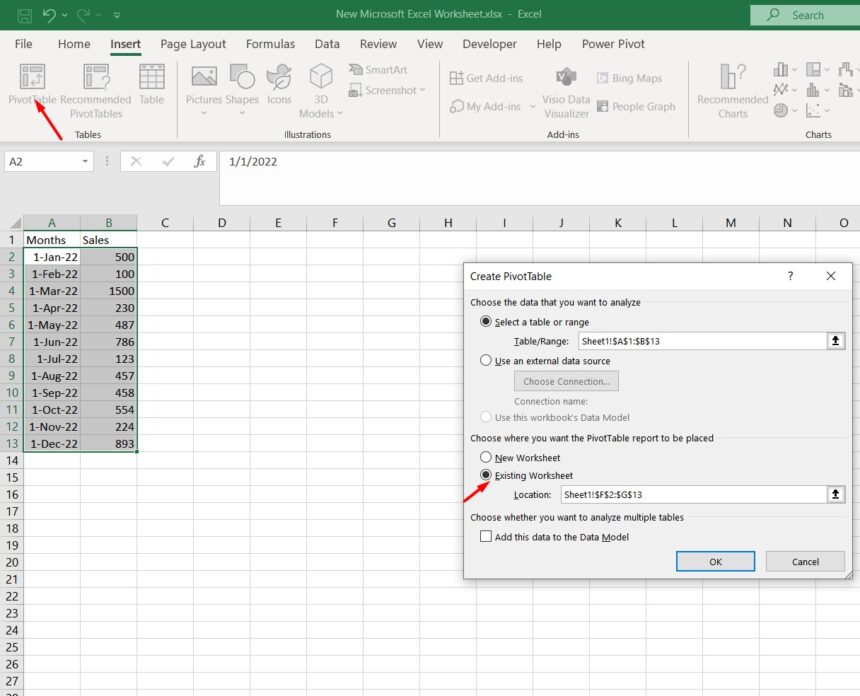
Step 1: Insert, Pivot Table is invoked by selecting one cell in the data and pressing the Insert, Pivot Table button. In the Add, This Data To The Data Mode section of the Create Pivot Table dialog box, choose the option to include the data in the data model.

Step 2: Insert the pivot table from the Insert tab on the reason, and you can select to display the table on the same sheet or a different sheet. If you choose the same sheet, you will have to give the range where you want the Pivot table. 
Step 3: After inserting the table, nothing will be shown until you check the boxes on the right to show the data you will be using. And just like that, your data will automatically be calculated in how to calculate rolling 12 months in excel.

How To Calculate Rolling 12 Months In Excel Using The Autofill Handle
How To Calculate Rolling 12 Months In Excel Using The Autofill Handle
The autofill on the handle in MS excel is a live saver. It has tons of features and can be used to make work very simple. We can use the autofill option to fill in the months automatically. We will show you how to do this task.
Step 1: Open up a new MS sheet, enter the first month with data, and drag the autofill handle until date 12. Next, click on the + sign at the bottom of the autofill handle.

Step 2: Now choose fill months, and excel will calculate the rolling 12 months in excel for you.
How To Calculate Rolling 12 Months In Excel Using Fill Series
The fill series can also be another way to easily insert a rolling 12 months in excel. You will only need to enter the beginning date, and the rest will be done in excel. The fill button can be found in the home tab.
Step 1: Open up a data sheet and enter the starting date. Select the number of months in the cell that you wish to display.

Step 2: Head over to the fill button on the upper right side of the Home tab, click it, and it will show you a popup box. You will need to select months from here and click okay, and your rolling months will be visible.

Calculating Rolling 12 Months In Excel By a Formula
Excel has a lot of functionalities, but most of them can be employed by using special formulas. These formulas can make your work easier by doing most of your work. You will just need to insert the formula in a cell and drag it till you get your desired months. The formula we will be using for this is “=DATE(IF(MONTH(A2)+1>12,YEAR(A2)+1,YEAR(A2)),IF(MONTH(A2)+1>12,MOD(MONTH(A2)+1,12),MONTH(A2)+1),DAY(A2))”
Formula Description
In this case, MONTH(A2)+1 signifies the month after the month of A2. So, for example, June will be represented as MONTH(A2)+1 when A2 includes May as its month value.
However, if the month in cell A2 is January, which implies MONTH(A2)=12, we will be unable to utilize MONTH(B4+1)=13 to advance to the next month. So we’ll have to start again at the beginning of the year with the year raised by one in such a situation.
The two IF functions included inside the formula do the same thing.
If MONTH(A2)+1 is less than or equal to 12, IF(MONTH(B4)+1>12,YEAR(A2)+1,YEAR(A2) returns the same year, and if MONTH(A2)+1 is higher than or equal to 12, IF(MONTH(A2)+1>12,YEAR(A2) returns the next year.
If the current month is anything other than December, the condition IF(MONTH(A2)+1>12 is satisfied; otherwise, it returns the next month as January. Likewise, if the current month is anything other than December, the condition IF(MONTH(A2)+1>12 is satisfied; otherwise, it returns the next month as January.
Finally, the year, month, and date are all included inside a DATE() function to get the whole date.
Step 1:
- Open up an MS excel datasheet.
- Enter the data according to your preferences.
- Enter the formula below that cell, and press enter.

Step 2: Next, drag the autofill handle until your required months to get the formula to work for you.
Conclusion
Now you know quite a few ways to calculate rolling months in excel easily. These tips and tricks will save your time and make you quite efficient. You should practice these techniques and if you face any problems let us know.