While Dealing with user names and other names or user IDs in general, we often face the problem of garbled text, and garbled texts in a large excel Spread Sheet can be bothersome. So we will learn how to remove this pesky character from excel spreadsheets. If you deal with usernames and other large excel spreadsheets, then Excel Remove First Three Characters is an excellent article.
We can deal with this problem in three easy ways. First is the Right Function, the Second Is the Replace Function, and the third is the Mid Function. These functions serve the same purpose, and you can use whichever Function you feel comfortable with.
Right Function:
The RIGHT Function combined with the LEN function will help us get our desired results of Excel Remove First Three Characters. 
1st Step: Open an excel file and enter the data you wish to remove the first three characters. We have entered our data into B Column. Our Formula Is “=RIGHT(B3,LEN(B3)-3)”
2nd Step: Take a Column where you wish the results to show. Now write =RIGHT, Start Parenthesis click on the first cell that contains the data. In our case, it’s B3. Now follow up with a comma and write LEN. A parenthesis will Appear now again. Select the cell with the data and type -3; close the first parenthesis and press enter to see the results.
3rd Step: You Should see the results as soon as you press enter and drag the result cell downwards to apply the Formula to the rest of the data.

Note: You can use the Formula to remove any number of desired characters from the data by using your desired number after the – Sign.
Replace Function:
The replace function replaces the date from one cell with different data, but we can use it to remove the first three characters quite easily. 
1st Step: Begin by applying the REPLACE Function C3. The Formula is “=REPLACE(B3,1,3,””)”
2nd Step: B3 is the cell where we will replace the characters. Start_Num is 1 because we are beginning from the start. Num_Chars is 3 as we are going to replace three characters. We are going to use double “ to signify the returned text.
3rd Step: Press enter to get the results, and you can drag the result cell downwards to apply the Formula to the rest of the data.
Note: You can use any number in the Num_Chars to replace the desired amount of characters you need to replace.
Mid Function
The Mid Function is more or less like the Right Function. You must use it with the LEN function to get the desired result of removing characters from data. 
1st Step: Let’s Start by applying our Formula =MID(B3,4,LEN(B3)-3) into cell C3.
2Nd Step: Here, B3 is the cell we wish to replace the text. Start_Num here is 4 because we with to remove the first three characters. Num_Chars is signified by LEN(B3)-3). We have now successfully entered the formula, and now press enters to see the results.
3rd Step: Like the rest of the techniques, drag the result cell or formula cell downwards to apply the Formula to the rest of the data.
Note: While trying to remove more characters, remember to change the number before LEN because this Function removes characters from the middle. You also need to count plus 1 while using mid Function.
Conclusion:
Now we have learned how to remove unnecessary characters from excel. These techniques will help us eliminate unwanted data from valuable data. This function will with people who work long order spreadsheets, spreadsheets lots of zeros, and with repeating data in any big spreadsheets.