This piece will demonstrate how to create a student progress excel spreadsheet. You will be able to track a student’s development throughout each term by using this template. The difference in grade point average (GPA) between the actual Grade received, and the Grade that was aimed for will also be calculated when determining the overall performance of every student. The information on the students’ overall performance and the number of unsuccessful students and the number of successful students will be plotted in the performance over time graph so that the development of the students may be seen.
Grading System For student progress excel spreadsheet
I have inserted the grades and grade points data depending on certain numerical values into this worksheet that I am using. You are free to implement your grading system in this section. After finishing the table for the grading system, I went to the Name Manager under the Formulas tab and established two name ranges for the GradePoints and Grade columns. These ranges may now be used.
Name List with Identifier and Grade Point Average Worksheet

This is the worksheet in which you will add the information about your students. The information on the student includes his ID, name, and current grade point average. The information in my table pertains to twenty-three different pupils. There is no limit on the number of students who may be enrolled in your class. Therefore, compile a list of every pupil. After gathering all the information, I went into the Name Manager and created two name ranges: one for the ID, and another for the List.
Worksheet with Grades and Numbers to List
On this worksheet, you will discover all of the information on the students, broken down into specifics. You will see that the other information in the student information section is automatically updated depending on the student ID after adding the IDs in the ID column. This occurs because the student ID is being used as a key. You can quickly input the ID into the cells of the ID column since they are equipped with a dropdown list option. You can only put data into the ID column, the first three Number columns, and the third Number column on this worksheet. I determined the overall score for the final assessment by giving each of the Midterms equal weight (20%) while giving the Final Term a weight of 60%. If you just have one midterm, you will be able to change the overall assessment outcome by altering the formula in the Number column of the very last column. If you wish to deal with one or multiple midterms, you may delete the columns or add new ones. When you have finished compiling the final assessment result, you will be able to see the number of students who passed and failed each term. Formulas are used to produce these. Suppose you want to determine which students received an “A+” after the course was completed and checked. To do this, pick the Grade located next to the Highlight a student’s information following the section under “Final Evaluation.” After completing the final assessment, the students who have received an “A+” grade will have their rows highlighted with green lines.
Note: Remember that the worksheet must be unlocked before any changes can be made since it is set to be locked by default. When it is locked, you will only be able to use the ID and the first three numbers.
Examine the worksheet’s dropdown menus to see whether you have inadvertently altered the Grading System worksheet or the Name List with the ID and CGPA.
Worksheet to Analyze Student Performance 
In this worksheet, you will see a column under “Performance,” which contains a formula for determining each student’s performance in each term. The calculation compares the student’s “Achieved Grade” to their “Targeted Grade.” Conditional formatting has been given to the columns labeled “Performance” (AG-TG) to make it simpler for you to monitor how the performance is changing. The sum of the values in this column will be used to assess the overall performance of the students each semester. It is computed in the row that contains the overall performance. Most of the fields on this worksheet are connected to the Grade and Number List worksheet; however, the columns labeled ID and Targeted Grade are missing from the latter. There is no protection on these two columns’ cells, even though they include dropdown menus. As a result, the only place you may enter data while the worksheet is protected is these two columns.
Note: Remember that the worksheet must be unlocked before any changes can be made since it is set to be locked by default. When it is locked, you will only be able to access the ID and the first three Targeted Grades.
Examine the worksheet’s dropdown menus to see whether you have inadvertently altered the Grading System worksheet or the Name List with the ID and CGPA.
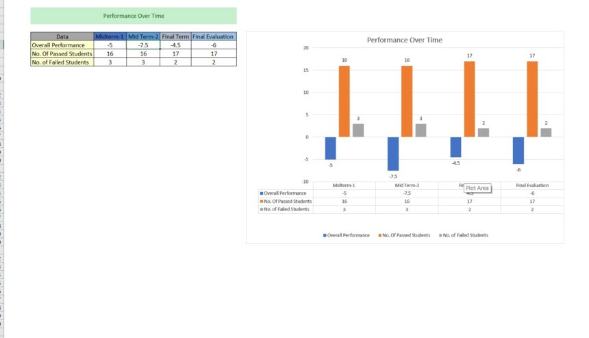
Worksheet Displaying a Graph of Performance concerning Time

You will find a graph titled “Performance Over Time” in this worksheet. This graph will be based on the overall performance of the students, the number of students who passed the test, and the number of students who did not pass the test. These values are connected to the worksheets titled “Student Performance Worksheet” and “Grade and Number List Worksheet.” Therefore, if you alter any of the values in these worksheets, the values on this worksheet will also change.
Conclusion
After reading this post, you will better understand how the template above will function. However, make sure you download it before you forget. This was developed especially for instructors to have an easier time calculating the results and assessing their student’s progress during each term. I hope that you like reading this essay. In the comment space below, kindly provide any recommendations you have for how we may make this template better, and kindly let us know your opinion.