In our excel lesson today You will learn how to quickly and easily sum several columns in Excel based on a single or many criteria by following the steps in this article.
As long as all of the numbers that need to be summed are contained inside a single column in Excel, doing a conditional sum is a piece of cake. The difficulty with adding several columns is that the SUMIF and SUMIFS functions need the sum range and the criterion range to be the same size. This makes it difficult to add up many columns. There is always a way around a problem, which is a blessing in situations when there is no obvious solution:)
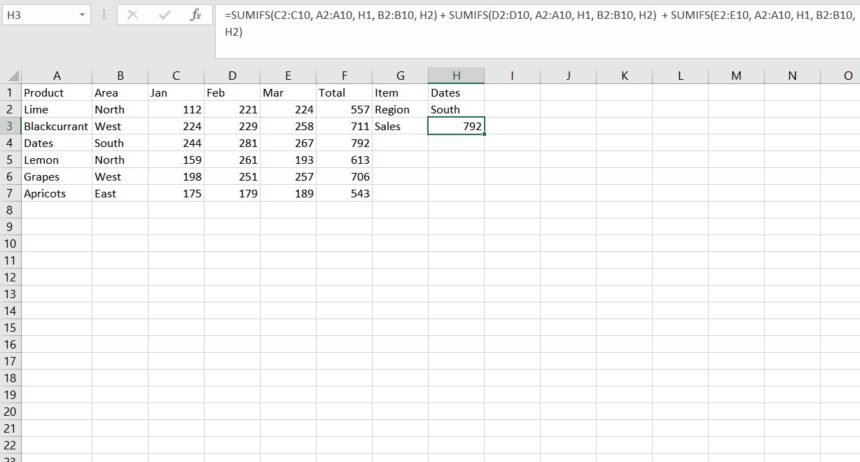
First things first, let’s figure out precisely the issue we are attempting to fix. Imagine that you have a table of monthly sales similar to the one displayed below. In addition, there are a few entries for the same product since it was combined from a variety of regional reports; these records are as follows:
The issue that has to be answered is: how do you calculate the total number of sales for a certain item?
The very first thought that occurs to me is to make use of a SUMIF formula in its unadulterated form:
=SUMIF (A2:A10, “dates”, C2:E10)
I’m sorry to say that this won’t be successful. This is because Excel will automatically calculate the dimensions of the sum range based on the dimensions of the range input. This is the explanation for this. Because there is just one column in our criterion range (A2:A10), the same is true for the sum range (C2:C10). In practice, the sum range parameter specified in the formula (C2:E10) just defines which cell in the range’s top left corner will be added together. As a direct consequence of this, the calculation above will only total the sales of apples in column C. Not quite what we were hoping to find, is it?
Sumif For Multiple Columns
Create a helper column that totals the values in each row individually, and then use that column for the sum range operation. This seems to be the easy and effective approach that can be found. So we will use this formula for the task. “=SUMIF(A2:A7, H1, F2:F7)”
Step 1: Open a Ms excel Sheet, enter the test data, and select a cell that enters the search query; here, H1 is the location for the search query. Then take another cell, apply the formula, and modify it to your needs.

Step 2: After modifying the formula, press enters to get the results. Then, you can change the query in H1 to your requirements.
Note: When there are a decent number of columns, this works as expected. However, when there are many columns, the formula becomes excessively lengthy and is difficult to understand. In this particular scenario, the alternatives that are listed below are preferable.
Sumif For Multiple Columns With Multiple Criteria
To sum the cells that match multiple criteria, you normally use the SUMIFS function. The problem is that, just like its single-criterion counterpart, SUMIFS doesn’t support a multi-column sum range. We write a few SUMIFS, one per column in the sum range to overcome this. We will find out the sales for dates from the South area. The formula we will be using is “=SUMIFS(C2:C7, A2:A7, H1, B2:B7, H2) + SUMIFS(D2:D7, A2:A7, H1, B2:B7, H2) + SUMIFS(E2:E7, A2:A7, H1, B2:B7, H2)”
Step 1: Use the previous data, enter the item names and the Area names in two cells, and enter the formula in the third cell. Apply the formula and modify the ranges. 
Step 2: After applying the formula, it will get you the results. Now, all that you need to do is change the queries for different items.
Conclusion
You know how to use sumif for multiple columns; you can use these to find your desired data from the data range, which you need in a few simple steps. Knowing these can make your work and life easier as you can find the data you want from a range of data easily and analyze them in no time. You only need to understand the ranges and enter them properly for these formulas to work.