Excel has a number of various formulae that may be used to VLOOKUP return multiple columns at once and return data from several different columns. Additionally, Excel possesses several formulae that can return data from a single column. To finish our calculations, we will need to combine the VLOOKUP function with an array formula. This is because the VLOOKUP function cannot independently extract many separate bits of data. In addition, there are several straightforward variations to the array formula that may provide results based on the contents of many columns. This article will provide a comprehensive analysis of each of these methods and relevant illustrations and photographs.
VLOOKUP Return Multiple Columns At Once With Array Formula
The next picture shows a dataset that is laid out, and it has a variety of smartphone models, each of which is accompanied by a list of their specifications. The table that is outputted at the bottom of the page will include all of the specifications for the smartphone model that is being viewed. We will use the VLOOKUP function to extract data from many columns for the mobile phone or smartphone device that has been supplied to us.
Step 1: Assuming that we are interested in obtaining the technical details for the 11t Pro smartphone gadget. The formula for the necessary array, which will use the VLOOKUP function in the output cell C15, will be as follows: “=VLOOKUP(B15,B5:F12,{2,3,4,5},FALSE)”
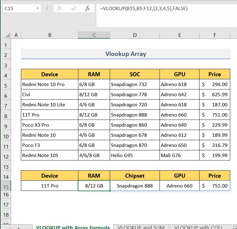
Step 2: When you hit the Enter key, the function will immediately return all of the specifications for the device you have chosen all at once. You can change the query in the b15 cell to look up different phones.
VLOOKUP Return Multiple Columns At Once With Sum
lookup Return Multiple Columns At Once With Sum
When the VLOOKUP function has finished returning values from many columns, we can do whatever type of calculation we want on the returned data. For example, the following data table provides the sales numbers obtained over five consecutive days for various salespeople. These sales figures were acquired over five days. In this specific scenario, we will search for a salesperson in the data table, extract the sales that correspond to that seller over five days, and then evaluate the total sales in the output column C18. This will be done since the case calls for it.
Step 1: Assuming we are interested in Ratul’s overall revenue, we should know the following. In cell C18, the necessary formula, which should include the SUM and VLOOKUP functions, should be as follows: “=SUM(VLOOKUP(C17,B6:G15,{2,3,4,5,6},FALSE))”
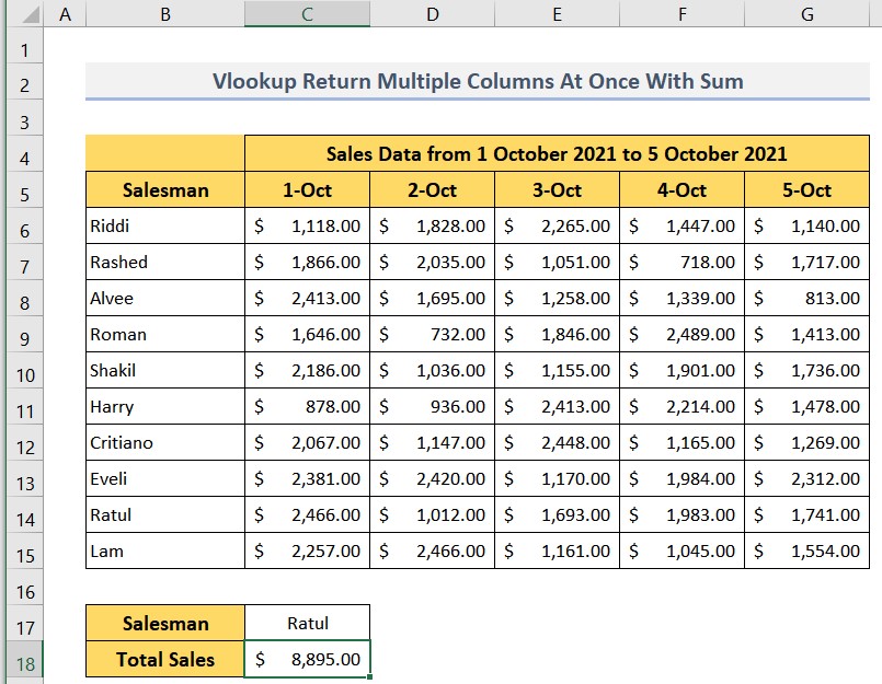
Step 2: Now hit Enter, and you will immediately be presented with the entire amount of money made by the chosen salesperson. Change the query to see results for a different salesperson.
VLOOKUP Return Multiple Columns At Once With Column Function
This time, rather than utilizing the array formula, we will employ one of the several available approaches to apply the VLOOKUP function in such a manner that it will generate numerous columns. Again, this will be done instead of the array formula. Rather than that, we will utilize the COLUMN argument of the VLOOKUP function to specify the column number in this specific case. After that, we are needed to utilize the Fill Handle that is positioned along the row to fill in the rest of the data for the mobile phone that has been specified.
Step 1: Given that we intend to extract the specs for Civi, the formula that has to be entered into the output cell C15 will be as follows: “=VLOOKUP($B$15,$B$5:$F$12,COLUMN(C$4)-1,FALSE)”
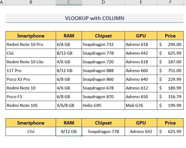
Step 2: Following is a list of the return values that may be found after hitting the Enter key and sliding the Fill Handle rightward till the very last output cell.
VLOOKUP Return Multiple Columns At Once With Index Match
The most effective alternative to the VLOOKUP function that is presently available is a combination of the INDEX and MATCH functions. This is the case since both of these functions are index-based. The INDEX function will return a value or a reference situated at the place where a certain row and column are crossed. This intersection may be any row or column in the data set. When the MATCH function is used on an array, it returns the relative position of an item in the array that matches a certain value in a defined order. This information may then be used in further processing. We will include the MATCH function that we have just acquired into our computation so that we may choose the row number for the lookup device.
Step 1: Suppose we want the data for Redmi note 10. Therefore, the necessary array formula for output Cell C15 will be as follows: “=INDEX(B5:F12,MATCH(B15,B5:B12,0),{2,3,4,5})” And the search query will be Redmi note 10 in B15.
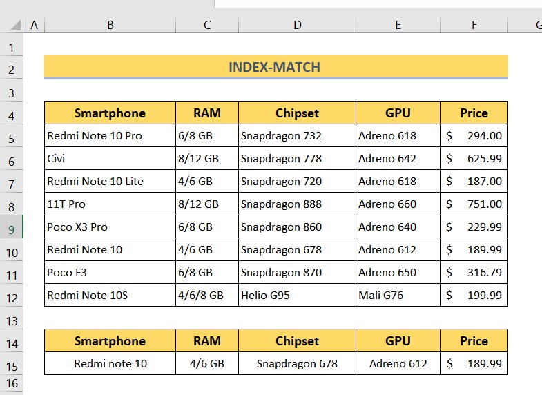
Step 2: After clicking Enter, you will be presented with a list of the chosen smartphone’s specs, which have been compiled from the information in various columns.
Conclusion
When you need VLOOKUP return multiple columns at once from a data table, I hope that all of these methods that were discussed above will now allow you to apply them in your Excel spreadsheets. If not, please let me know so that I may make this information clear. I would ask that you use the comment box to interact with me about any questions or ideas that you may have. You may find that reading any of the other articles on this website linked to Excel functions also interests you.

