In order to establish a VLOOKUP or HLOOKUP function, you will need to input a range of cells, such as D2:F39, in the appropriate boxes. This range is referred to as the table array argument, and an argument is just a data component that a function requires in order to carry out its intended operations. In this instance, the function will go through those cells to see whether they contain the data that you are looking for.
The value you are looking for is always the first parameter in a VLOOKUP or HLOOKUP function; the table array argument comes after the value you are looking for and is required for the functions to be successful.
Your first parameter, the value that you wish to locate, maybe a particular value such as “41” or “smith,” or it can be a cell reference such as F2. Both of these options are acceptable. The first point of contention may thus be stated as follows:
=VLOOKUP(F2, …
The table array parameter will consistently come after the lookup value in this format:
=VLOOKUP(F2,B4:D39, …
The table array option may make use of either relative or absolute cell references for the cell range that it specifies. You need to make use of absolute references in a format similar to this if you want to duplicate your function:
=VLOOKUP(F2,$B$2:BD$39, …

Additionally, the cells that make up the table array parameter may exist on a different page inside your workbook if you so want. In such case, the argument will include both the name of the sheet and itself, and the syntax will look like this:
=VLOOKUP(F2, Sheet2!
$C$14:E$42, …
After the name of the sheet, you should put a point after the exclamation point.
You are now at the point where you have to input a third parameter, which is the column that holds the data that you are attempting to locate. This column has been designated as the lookup column. In the first example that we will look at, we will be using the cell range that spans three columns and goes from B4 to D39. Let’s imagine the numbers you’re interested in are located in column D, which is the third column in that range of cells; hence, the last argument will be a 3.
=VLOOKUP(F2, B4:D39,3)
You have the option of using the fourth parameter, either True or False, but it is not required. You should go with False the vast majority of the time.
If you specify True or leave the fourth parameter unspecified, the function will return a value that is a close approximation of the value you specified in the first argument. In order to continue the demonstration, let’s say that the first input you provide into the function is “smith.” If you then pass True into the function, it will return results such as “Smith,” “Smithberg,” and so on. However, if you use the value False, the function will only return “Smith,” which is an exact match, which is what the vast majority of people want.
If your lookup column, which is the column you indicate in your third parameter, is not sorted in ascending order (from A to Z or from lowest to highest number), the function may return the incorrect result. This adds an additional layer of complexity to the use of True. Look up data using VLOOKUP and other methods for further information on this topic.