Let’s pretend that we have access to a dataset that includes the information “Distance covered by various participants during a marathon.” There are a few blank spaces at the end of each Participant Name, and the cells in the Distance Covered column have the numerical values in addition to the unit of miles. Now that we’ve gotten that out of the way, let’s go on to trimming the spaces and the characters that denote the unit from the right.
When dealing with unstructured text data in your spreadsheets, you will often be required to parse the data to get the information that is pertinent to your job. You will learn how to delete any number of characters from the left or right side of a text string by reading this article, showing you a few basic techniques.
Trim From Right Excel Using Trim
At times, your data cells could have some additional spaces at the right end of the row. To get rid of these gaps, we may utilize the TRIM function. As was said before, there are a few blank spaces after the names of each Participant. We can use this function to remove empty spaces from the string. We have added numbers and symbols to the string to show the removal of empty spaces. The formula is easy “=TRIM(A2)”.
Step 1: Open an MS excel file and enter the data or use your data and select an adjoining cell to enter the formula.

Step 2: Modify the formula to your data and or place the formula and press enter, and the formula will remove the characters from the right.
Trim From Right Excel Using Text To Columns
You may also utilize the functionality of Text to Columns to trim the appropriate spacing in your document. This approach will need an empty column to the right of the column, which will serve as the location from where the spaces will be removed. To begin, add a column immediately to the right of the column from which you will be removing the space. Excel’s built-in functions can do a lot of work if you know what to do. We will show you how to employ these to Trim From the right excel.
Step 1: Open an MS excel file, select the data range, head over to the Dataribbon’s tab, andd select Text To columns.

Step 2: From the popup box, select fixed width, press next, fix the width, and press finish. The Text and the remaining string will be shown in two columns.
Trim From Right Excel Using Len
By combining the LEFT function with the LEN function, it is possible to simply remove the the right characters from your worksheet’s data cells. Enter the formula shown below into a currently empty cell (A2). The LEN(A2)-5 portion of this formula indicates that the last six characters of the total length of cell A2 will not be included in the return of the LEFT function. The LEFT function indicates that the formula will return the characters of the selected cell, which is A2, from the LEFT portion of the formula. So the whole formula for this function will be “=LEFT(A2,LEN(A2)-5)”
Step 1: Open the previously used excel file, remove the old data, and insert new data.

Step 2: Then apply the formula in the next cell, press enter to see the results, and drag the autofill downwards to apply the formula to the rest of the data.
trim from right excel For Numbers
The output will always be in the form of Text regardless of which of the following formulae you apply, even if the returned value just comprises numbers. Either includes the core formula in the VALUE function or does any mathematical action that does not alter the result, such as multiplying by one or adding zero. This will allow you to return the result as a number. When doing further calculations based on the findings, you will find that this method is quite helpful.
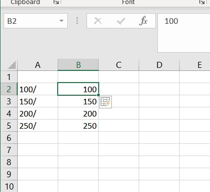
Imagine that you have eliminated the initial character from the cells A2:A4, and now you want to add up the values left behind. Surprisingly, the result of a simple SUM calculation is always zero. Why would that be? The obvious reason is that you are adding up strings rather than integers. If you carry out any of the procedures listed below, the problem will be resolved! So extracting the numbers from a string requires the formula “=RIGHT(A3, LEN(A2) – 1) * 1” This formula will clean up your text strings and get the numbers from the range. This is quite useful when dealing with id nos.
Step 1: Open an Excel File, enter the data, apply the formula in an adjoining cell, and modify the range.

Step 2: You can now press enter to see the results, and you can drag the autofill handle downwards to apply the formula to the rest of the range.
Trim From Right Excel Using Flash Fill
The Flash Fill tool is available in Excel 2013 and subsequent editions, and it is another straightforward method for deleting the initial and final characters in an Excel cell.
Step 1: In the cell next to the first cell containing the original data, input the desired result while leaving out either the first or the final character from the originally entered string, and then hit the Enter key.
Step 2: In the next cell, begin entering the anticipated value. Excel will provide a preview of your data without the first or final character if it detects a pattern in the data you are entering and will follow that pattern in the remainder of the cells if it finds a pattern in the data you are entering. To continue, just press the Enter key on your keyboard.
Conclusion
Excel allows you to use any of the aforementioned ways to trim from right excel. Leave a comment below if you’re having any trouble understanding anything. In addition, excel allows users to delete a substring from the left or right side by following these steps. In closing, I’d want to state that each of the approaches mentioned earlier is quite simple and uncomplicated to practice.
The first three ways are based on dynamic formulae. On the other hand, the text-to-column approach is rapid, but it requires you to apply it repeatedly, which may make it less useful at times.