In this recurring deposit calculator excel guide, I’ll demonstrate how to use Excel to compute compound interest, also known as the maturity value, for recurrent deposits. It will be difficult to save money if you do not have a strict financial plan. But there are many reasons why conserving money is crucial in life. We would like to preserve:
- To be used towards our contingency fund.
- Because you freed us from the burden of debt.
- For our retirement
- For the sake of the education of our children
- And to amass wealth
Putting money aside might be challenging for some individuals. An excellent choice for individuals in this category is opening a savings account, establishing a monthly automatic deposit, and waiting a few years for the balance to grow to a respectable level.
This recurring deposit, also known as an RD, is a common savings method across the Indian subcontinent. As someone who hails from Bangladesh, I can attest to the widespread adoption of the recurring deposit (RD) system.
The following are some of the reasons why Recurring Deposit (RD) is so popular:
- Monthly savings opportunities are available for those who choose to invest.
- They are compelled to set aside money every month thanks to this plan.
- Guaranteed and risk-free profits from their investments.
- Within the framework of this plan, one pays little or no income tax.
Allow me to now walk you through calculating the value of your maturity for the regular deposits using Excel. First, it is a good idea to understand how everything about your investment works. Then, you should never be in the dark when it comes to your financial situation.
FV Function For recurring deposit calculator excel
The FV function can calculate the future value of an investment by using recurring payments at a fixed rate of interest to determine the worth of the investment in the future.
The FV function’s syntax is as follows: FV (rate, nper, pmt, pv, type)
Here,
- rate: The rate of interest every month
- nper: The total amount of periods
- pmt: The amount paid at the end of each period
- pv: Present value type: Form or manner of payment. There are two possible timings for payments: (1) at the start of the period and (2) at the end of the period (omitted or 0).
I have incorporated the FV function into this particular approach.
You can see that there is a column for the input values. The following values will need to be entered by you:
RD stands for recurring deposit. The amount you will put away every month (or any period). We gave this cell the name pmt.
Payment Frequency: It is a list that you may select from. The majority of the time, it is every month. However, the drop-down menu allows you to choose any period.
We have also estimated the number of periods per year (npery) using the VLOOKUP function in Excel. The formula for this can be seen on the right: =VLOOKUP(C7,periodic table,3,0). The periodic table will be provided for you in the worksheet titled “Tables.”
The total amount of time in years you plan to continue making deposits into your fund. When we multiply the total number of years by the average number of periods in a year, we can calculate the total number of periods, denoted by the symbol nper on the right (npery).
The Annual Percentage Rate, often known as the APR, is the basic interest rate your bank is willing to give you.
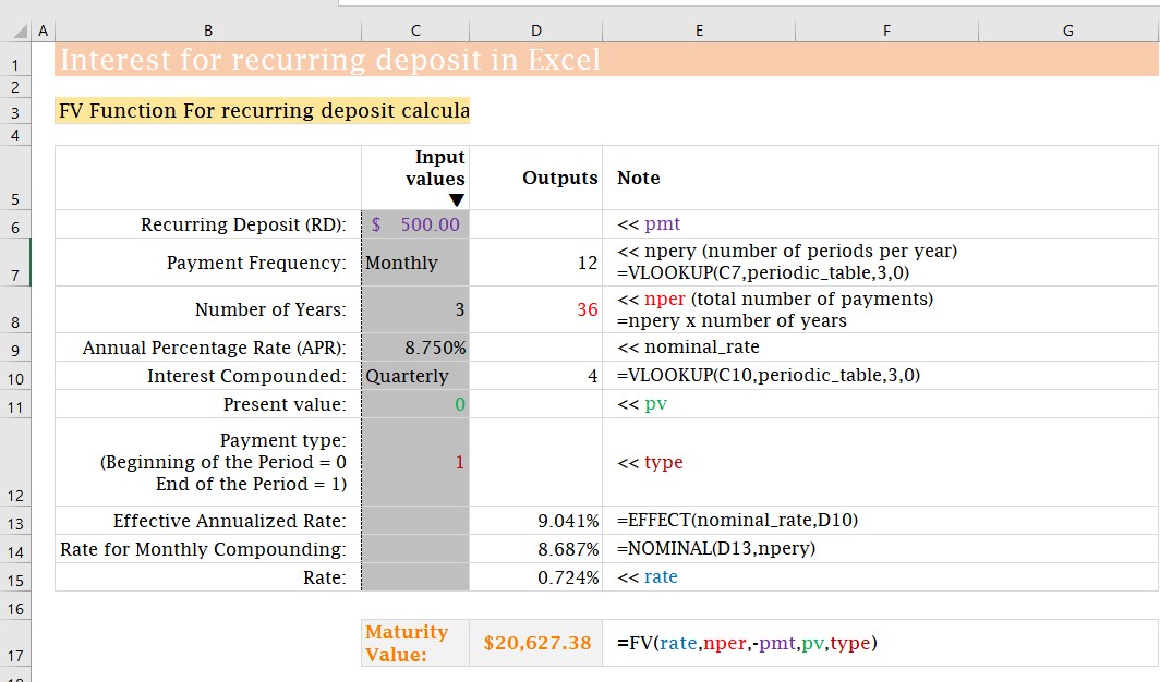
Your investment receives interest compounded every quarter by Indian Banks. There may be variations from bank to bank. This is another list that may be selected. Therefore, you can select any compounding frequency.
Keep in mind that the frequency of your interest being compounded needs to be either equal to or larger than the frequency of your payments. Therefore, you cannot select the Weekly, Bi-weekly, or Semi-monthly options for the Compounding Frequency value, for instance, if the Payment Frequency that you have selected is Monthly.
You can see the number of times compounding has occurred annually in the right-hand column. We were able to find it by utilizing the VLOOKUP tool in Excel: =VLOOKUP(C10, periodic table,3,0)
After that, you will need to enter the Present Value and the Payment Type (either 0 or 1).
Here comes the most difficult part:
The frequency of our recurring deposits is monthly, whereas the frequency of our compounding is quarterly (or any).
The question now is: how will we approach this predicament?
What we require instead is the same rate on an annualized basis. Therefore, the following steps need to be taken to compute the actual rate for quarterly compounding: =EFFECT(8.75 percent,4) = 041 percent.
We need a nominal rate that, when combined with monthly compounding, will give us the same effective rate: =NOMINAL(9.041 percent,12) = 8.687 percent. You may double-check it by doing it in the following way: determining whether or not this nominal rate of 8.687 percent will generate the same effective rate with monthly compounding: =EFFECT(8.687 percent,12) = 041 percent. Same.
Now that we require the rate for a specific period (monthly), we may calculate it as follows: 687 percent divided by 12 equals 0.724 percent. Finally, we will attach the Template. You will only need to enter your data to get the results you are looking for.
Direct Method For Recurring Deposit Calculator Excel
Calculating the Maturity Value of your Recurring Deposit (RD) for 36 periods will need the following series of step-by-step instructions (3 years).
In this instance, we have maintained the same pmt value and the same rate each period. However, the process is straightforward. Let me clarify.
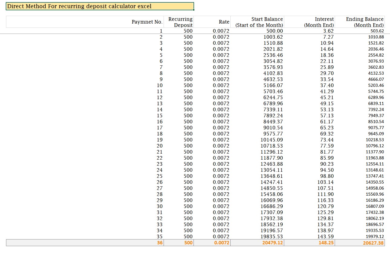
An explanation of the picture is as follows:
You deposit $500 at the beginning of each month. You will get an interest payment of $3.62 at the end of each month due to the investment. Therefore, your final balance is $500 plus $3.62, which is 503.62
You deposited an additional $500 at the beginning of the second month, and your balance after the previous month was $503.62. Therefore, your total Beginning Balance at the beginning of the second month is $503.62 plus $500, 003.62 dollars. On this sum, which is $1003.62, you will receive interest for $7.27 every month. Therefore, your ending balance will be $1003.62 plus $7.27, 1010.88 after the second month.
The table moves forward in this manner.
Simply copy the last row of this table and paste it at the level where you want the additional periods to appear.
Conclusion
You have gained a very valuable lesson from the recurring deposit calculator excel567 if you have read this text in sequential order from beginning to end. Before I started using Excel, I had a lot of trouble calculating even the periodic deposits that my mom made and their Maturity Value. However, it is clear to me now how to proceed.
Therefore, this is the method that I use to compute the interest on regular deposits using Excel. What are your thoughts on the content of this article? How helpful was it? Have you been able to use my calculator without any issues?


If you provide the template it’s help a lot’s